
Welcome to my tutorial on getting the eigenvector of the mesh laplacian in Houdini.
I will describe:
- How to get started with the HDK in VSCode
- How to get a vague idea about eigenspaces
- How to go from C# to basic C++
But also attempt to describe:
- How you learn about a complicated topic by building a testbed for your own learning.
When I started with this I didn’t know anything about the Spectral Analysis, the Laplacian, Eigenspaces, C++, or the HDK.
I am not a mathematician and previously had not done any C++.
It is written mostly for the Technical Artist, who often has to learn and utilize concepts in short timeframes for some implementation. So I assume you know some C# and
have some understanding of 3D graphics and vector math.
Remember:
This is a starting point and the final outcome is not necessarily suited for use in production.
Motivation
This entire project came about after reading this blog post, which frequently circulates in the Houdini community:
https://houdinigubbins.wordpress.com/2017/07/22/fiedler-vector-and-the-medial-axis/
Understanding at least the concepts of this is what this article will be about and how I implemented it in a basic form in Houdini to actually see if what I thought was in any way correct.
The philosophy
I will focus on iterating in small steps and continuous testing to try and match my actual process when I was trying to understand this.
Research
The Math
The mesh laplacian,
is a matrix, unique to a mesh,
used to get the divergence of the gradient of any values.
It is approximated, most commonly with "cotangent weighting"
and inherently describes curvature.
The matrix is NxN in size,
N being number of points.

Eigenvectors are vectors which,
transformed by this matrix,
will only change magnitude.
These will be 1xN in size.
The laplacian is an operator which describes how to get the divergence of the gradient (or the “derivative of the derivative” or “rate of change of the rate of change” or to some extent “the curvature”) of a function in a specific context.
The laplacian is well described here.
Context here is not the scientific term, but think of it as “the kind of data” being worked with. If it is a heightfield, a mesh, a volume, a 2D function or a higher dimensional function. In each case the operator will be different. For example. For the mathematical function, it will be a transformation into a new function. For the heightfield (or image) it can be abstracted as a 3×3 image processing kernel, as it is uniformly applied (except for, literally, edge cases).
We would usually call this an edge-detection filter, though a simple one. This helps in understanding the laplacian as an indicator of value changes.

For the meshes, though, we need to use a definition which can vary between points. First, we will consider using a Laplacian Matrix. The approach to constructing the graph can be found on Wikipedia under the Example Section. It is a much larger datastructure, because each node, so each value, can be affected by a varying number of neighbour values. It is on this non-localized operator we can find the eigen-vectors.
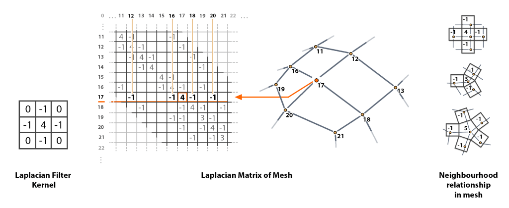
So we are simply talking about a way of applying the laplacian. Not the result of it, but the operator. In this case represented by an NxN, where N is number of vertices..
Do notice that in this form, positions of the vertices (the nodes) are irrelevant.
It is entirely a property of connectivity.
This is all fine and good, but this is not the Laplace-Beltrami ,
To go from the Graph Laplacian to the Mesh Laplacian, we need to introduce the concept of cotangent weighting, which is one of several methods, but this one is often preferred .
Cotangent weights describe the amount of deviation from a flat surface, based on the angle of the adjacent triangles. You could find the averaged plane of the surface, but this would assume the point corresponds to the exact centerpoint between neighbours shifted up along the derived normal and would not be as precise an estimate. (Remember, meshes do not really have curvature, they are faceted. We are calculating an approximation of an interpreted underlying smooth mesh).
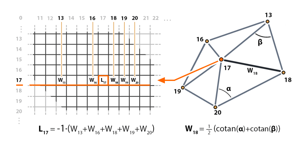
With this formula, we are ready to calculate each entry for the cotangent laplacian matrix.
As an additional bonus is remembering that even when involving trigonometric functions, if you are not going from linear to angular, but really linear to angular to linear , there is usually a shortcut. In this case:
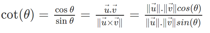
The interpretation of this is that, as the tangent is sine/cosine, the cotangent is cosine/sine.
The sine of the angle between 2 vectors is the magnitude of the cross product.
The cosine of the angle between 2 vectors is the dot product.
Note: We will be implementing a version that does not account for the vertex area, which would require scaling weights by the inverse of vertex area (weight / sum of surrounding primitives divided by 3). This is presumably because the matrix thus becomes non-symmetrical and requires a different solver from Spectra, which, at the time of writing, I could not make work.
The Eigen-vectors are vector, which only change in magnitude and not direction, when multiplied with the associated matrix. The eigenvalues is the amount they change by.
They represent a spectral decomposition of the topology when applied to an operator of the second derivative. Meaning each vertex will have a value in relation to its neighbourhood that matches a wave-like function.
The whole process is well described in this video.
This means the eigenvector can be broken down to a simple wave, much like with Fourier Series to solve PDEs.
We will try to get an idea about what the terms mean,
but we will test our understanding by doing an actual implementation.
In this way, we can actually figure out if the terms made sense or if we got them fundamentally wrong.
Firstly one will just start reading about the topic, trying to find out what the fancy math words even mean.
In this case, we can at least take a few hints from the article:
- Laplace-Beltrami
- Eigenvectors (Fiedler)
- Spectral Analysis
So what is the main question?
Well, the first question is what the Fiedler Vector is.
How do the other words relate?
Well, the Laplace-Beltrami
is a operator of which you can get an Eigenvector from.
Spectral Analysis
is something with the eigenvectors and eigenvalues of something .
The blog contains plenty more knowledge on the matter,
For the Spectral Analysis article, I went down the rabbit-hole of trying to understand the adjacent concepts too. It seemed like the big question were just the eigen-doodads, but the lesson here is to limit what answers you are looking for before also trying to “project the points” find out how it “relates to the Discrete Fourier Transform” or others of these concepts that might be small extensions, but would involve extra confusion and time spent. These are all extensions on top of your first question anyway. Try to stay focused. It will save you time!
The problem with understanding any of these math terms
is that they are usually described with more math terms!
Let us look up some of them.
- Laplace-Beltrami
- Discrete Laplacian
- Laplacian Matrix
- Algebraic Connectivity
- Graph Partitioning
- Spectral Clustering
Often you will be able to find several papers, either by students, researchers or lecturers,
which will drop hints of words you can use for cross-referencing.
- Fiedler’s Theory of Spectral Graph Partitioning
- Discrete Differential-Geometry Operators for Triangulated 2-Manifolds
- Numerical Mesh Processing
- Spectral Compression of Mesh Geometry
- Spectral Mesh Processing
- Spectral Methods 1
- Laplacian Mesh Processing
- Spectral Mesh Processing
Oftentimes there are also very helpful people out there who have gone through much effort to describe the terms that are easier to comprehend:
- Laplacian Intuition
- Eigenvectors and Eigenvalues
- Spectral Partitioning series
- Spectral Partitioning series
Just from the videos alone, we get a good basic intuition for the Spectral Analysis part.
The one thing we do not know is exactly is what kind of laplacian operator.
The Spectral Partitioning videos do mention the graph laplacian,
but we are looking for the “Laplace-Beltrami”.
So let us see what we find if we search for the “Laplace-Beltrami”:

Screenshot from this slide, page 28.
We already have a description of the Discrete Laplacian on Wikipedia,
and if we go here we can read this:
“For a manifold triangle mesh, the Laplace-Beltrami operator of a scalar function
u at a vertex i can be approximated as…”
Which we can back up with the wording in reference 8, p13:
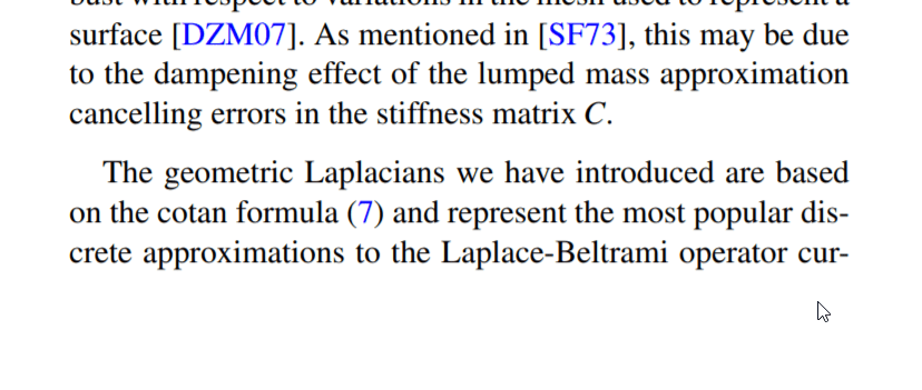
So from this, we can conclude that the cotangent operator gives an approximation of this Laplace-Beltrami.
A bit of searching will reveal plenty of information on the cotangent operator.
But a practical example is always better, like this one.
Now we have an idea about what is going on and also a method of calculating it.
If you want more clarity on what the cotangent weighting does,
you can find more information in the papers linked above.
Assumptions confusing me at this point were:
I knew what the laplacian is as something related to the Sobel operator, so a kernel of 3×3 entries.A vector is 3 or 4 coordinates long and is a property of a single point or pixel.
A matrix for transforming geometry is a transform matrix of 3×3 or 4×4 entries.
As you can tell, I had a very specific limitation on my view of geometric transformations at this point and had to remind myself how I had grown into a specific perception
The Programming
Basic difference between C++ and C#.
is the fact that one is compiled to machine code,
has a file structure to accommodate this compiling
and has manual memory management.
Where the other one is compiled to a runtime language,
has a structure more aimed at managing the code
and has memory management built in.
Header Files
Pointers
References
Stack/Heap allocation
C# and C++ have several things in common. They are both hard-typed and object oriented. However, C# is a much more modern language with more high-level features and easier syntax.
For example, C# uses the . for many different operations, where C++ use several symbols.-> for accessing a member of a class to which you have a pointer.:: to indicate that the left side is a namespace and the right side should be found within this namespace.
Passing by reference or by value is also fairly automatic in
C#, because you just pass by value!.. Unless you use ref or out.
In C++ you need be specific! You both have references, which are useful if you don’t want to copy the data to a new variable, but just want to reference it with that variable.
This is done with the variabletype& variablename syntax.
You can also have a variable, which is just the address of another variable. It isn’t a value in itself, it just points to this value. It is called a pointer and it is different from a reference. It is defined with variabletype* variablename.
Try not to confuse them with the address-of and the dereferencer symbols, assignee = &variablename... and assignee = *variablename...
Process
Whenever learning a new language, I take the approach of finding a simple example and trying it out.
In this case, the example were the samples in the HDK
Which is more complicated that preferable.
Using the inlinecpp python function
can help with that
as it can take away some of the surrounding code
and lets you focus on the core
Pointers, references and the fact that they use the same symbols confuse me, but knowing them is important. Especially if you try your hands at COPs or implementing OpenCL somewhere, where asking for the data in an image buffer won’t give you a nice class. It will not even give you an iterator, or an array.
No, you just get pointer to where in the memory the data is. Casting to the rightkind of pointer, incrementing it and not going out of bounds is all on you!
Setup
We need a Compiler and an IDE
Download and Install Visual Studio Code.
Download Build Tools for Visual Studio (Under "Tools for Visual Studio")
Follow this guide on setting up a C++ in VSCode.
For developing C++ we need an IDE, as in, a text editor with some basic tools for searching, navigating files, code completion and syntax checking. On top of this, it also handily has a debugger. Which will let us actually see what happened under the hood when the system crashes.
IDE’s like Visual Studio are getting very big and feature-rich, but this also means there are more bells and whistles to account for when setting it up.
Luckily, we have the choice of some more light-weight programs. One of which is Visual Studio Code. Visual Studio Code will work fairly easily with the right compiler, both being from Microsoft. It is also very minimalistic but easy to expand.
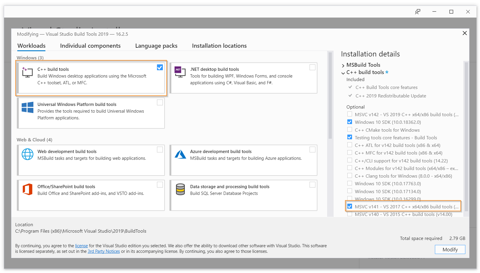
We also need a compiler, which is always dictated by the SDK we are developing with. In this case it is listed in the HDK documentation as being Microsoft Visual C++ 2017, version 15.8.5 (v141).
We can grab it independently from the Visual Studio download page

Upon installation, choose the right compiler in the list. The correct compiler version needs to be selected and the Windows SDK needs to be installed.
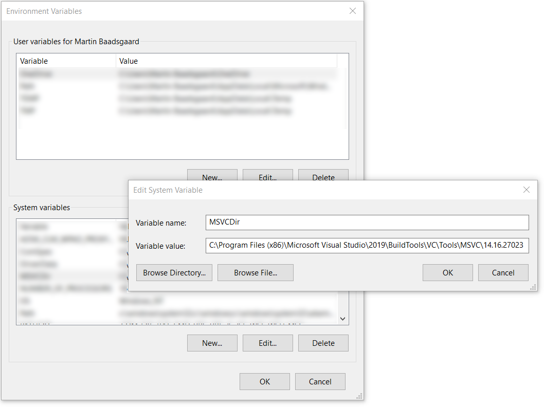
Another step, mentioned in the HDK, is to set the System Variable correctly. In my case it should be set to C:\Program Files (x86)\Microsoft Visual Studio\2019\BuildTools\VC\Tools\MSVC\14.16.27023
Process
When choosing an IDE, you might as well choose the one you are comfortable with. If that is “none so far” then pick the simplest that will get the job done. This goes back to the mentality of not adding anything before you got the core working.
The biggest question with VSCode was whether C++ would work, but there is a guide for that.
When choosing compiler, or any version of any system, try to match the one described. If it does not have the greatest features, that’s fine. You can port when you know it works.
Why Visual Studio Code?
I personally use Sublime as external editor with Houdini because it opens faster. However. Setting up C++ in VSCode was just so easy and I feel better recommending this because it also, very well, supports every language in Houdini, Including VEX! which is pretty sweet! It also behaved better with Python for Houdini in my tests.
We need an Eigensolver!
For the eigensolver we will use Spectra, which requires Eigen.
Go ahead and download the sources.
These are header-only, so they are very easy to include in the project.
Eigen is a library for working with matrices and Spectra is a library for finding the eigenvalues of large sparse matrices.
These two libraries can be downloaded and included with relative ease, as they are just a collection of header-files (not using the separation of definition and implementation the header/cpp files usual for C++ projects).
For souce, see above.
Process
As previously mentioned, there is also plenty of information on the original blog where we started out. For example here where the libraries Spectra and Eigen are mentioned.
So it is worth it to make sure you have exhausted your original source before going google-hunting.
It should be of no surprise that finding these names was what got this article started.
Had I been tasked with finding this solution, I would probably have stopped already at Eigen’s own eigensolver, not knowing any better. It would also have fitted with the philosophy I try to stick to with this project. However, I have a feeling I would have given up without Spectra.
Setting up a Development Environment
Set up a new project with Visual Studio Code.
Set the debugger to launch Houdini.
Compiling will be done with hcustom
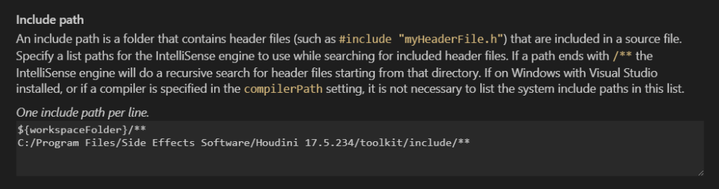
Once you have a project set up in VSCode, you can go ahead and copy in the files from Eigen and Spectra to the other includes at C:\Program Files\Side Effects Software\Houdini 1x.x.xxx\toolkit\include . Which we do as this eliminates a lot of problems with the linking.
We need to start a project, so use this guide to get a project set up (You do not need to create a build task, but you do need to set up the include path from the Houdini installation folder, for intellisense to work.
We also want the debugger setup, so we are able to catch any errors or crashes from Houdini. We can actually launch Houdini through VSCode’s debugger and if we compile with debug symbols, we can get the call stack and actually properly debug the plugin.

    "configurations": [
        {
            "name": "HoudiniDebug",
            "type": "cppvsdbg",
            "request": "launch",
            "program": "C:\\Program Files\\Side Effects Software\\Houdini 17.5.234\\bin\\houdini.exe",
            "args": [],
            "stopAtEntry": false,
            "cwd": "${workspaceFolder}",
            "environment": [],
            "externalConsole": false,
            "preLaunchTask": ""
        }
    ]
Process
This step is important because this is where we make sure to get functioning code, where we can test the effect of small changes fast. This is what will make it easy to try out if we understood things right, through trial and error.
The approach is a bit “dirty” and it would be better to set it all up with CMake and keep the libraries separate, but once again, it is added work for a proof on concept and just more things which can break
Setting up the Houdini scene
Calculate cotangent per half-edge opposite of corner.
Store on source vertex of half-edge.
Sum up the relevant cotan values per point.

Source file here
We will be triangulating our mesh with the remesh node, to get triangles and avoid obtuse angles. We can make the whole thing simpler by just using the number of connected points per point (the graph laplacian) but this would be a purely topological operator. (It kinda works though, thanks to sensible edgeloops in the model, if it is not remeshed)
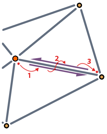
We will be using the cotangent of each triangle twice, for the vertex of each end We have to calculate the cotangent for each half-edge.
Each vertex will be the source of 1 half-edge, so we can use the source vertex to store the half-edge data.

Grabbing the destination of the half-edge we have the source for,
then the next edge,
then the destination of that,
.. will give us out 3 points in any case.
We subtract the points to get the 2 vectors, A and B.

Which we then use our previously found formula to get the cotangent of the angle from.
Put this in a Vertex Wrangle
int starthedge = vertexhedge(0, @vtxnum);
int nexthedge = hedge_next(0, starthedge);

int secondvtx = hedge_srcvertex(0, nexthedge);
int cotanvtx = hedge_dstvertex(0, nexthedge);

vector P1 = @P;
vector P2 = vertex(0, "P", secondvtx);
vector Pc = vertex(0, "P", cotanvtx);
vector a = P1-Pc;
vector b = P2-Pc;

f@cotan = dot(a,b) / length(cross(a,b));
To then calculate cotangent weight per point, we get all vertices associated with each point, as each will always be the source some some half-edge we need. To get the other cotangent, we…
- Get the half-edge of the vertex.
- Get next equivalent half-edge (There is always only 1 in non-manifold geometry)
- get the source of the half-edge
We grab both the cotangent and the point number it belongs to from the found vertex.
Put this in a Point Wrangle
int vertices[] = pointvertices(0, @ptnum);
int neighbours[];
float weights[];
float weightsum = 0;

foreach(int v; vertices) {
    float w1 = vertex(0, "cotan", v);

    int hedge = vertexhedge(0, v);
    int nhedge = hedge_nextequiv(0, hedge);

    int v2 = hedge_srcvertex(0, nhedge);
    int v2p = vertexpoint(0, v2);

    float w2 = vertex(0, "cotan", v2);

    float wfinal = (w1+w2)/2;

    push(neighbours, v2p);
    push(weights, wfinal);
    weightsum -= wfinal;
}
f[]@weights = weights;
i[]@neighbours = neighbours;
@weightsum = weightsum;
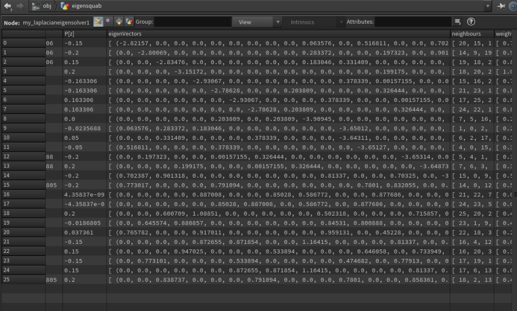
Lastly, our technique for storing the eigenvectors, will be an array on each point. This is because there will be 1 vector component per point in the geometry, so we store that component for every generated vector on the same point.
So we use a small wrangle node to write it into a test value…
@test = f[]@eigenVectors[1];
… Add a visualizer to highlight it after.
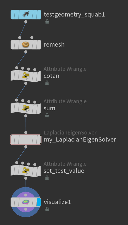
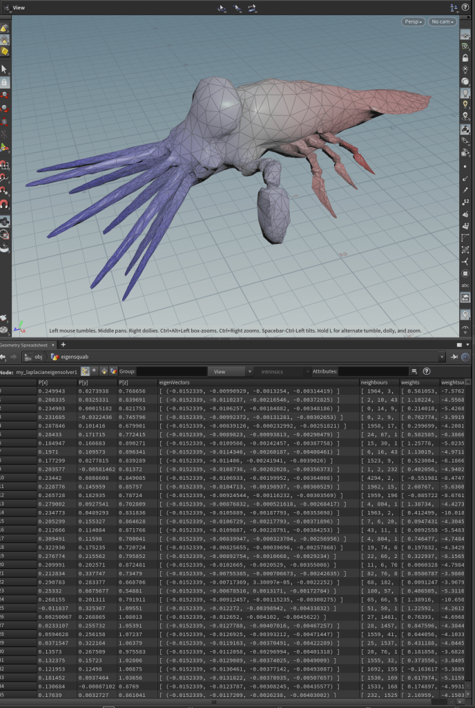
So this leaves us with:
- Remesh node to get a well-behaved triangular mesh
- Vertex Wrangle to calculate all cotangents per half-edge
- Point wrangle to sum up and average cotangents
- Our (not yet created) solver
- Point Wrangle, Copying out the second eigenvector (the Fiedler vector) to a test variable
- Visualize node to show the variable in the viewport.
Process
Setting up the Houdini scene takes steps out of the plugin creation and moves them into familiar territory. We know that what we do here can be done in the plugin, but we are unsure of how. To the extent that we would also not be sure whether we introduced any problems if we tried to implement it all in the plugin. Minimize the problem, minimize the steps.
The code for the cotangent was a shortcut borrowed from C++ but also initially implemented in VEX. If it works there, it means we understand it and can move it to C++ again afterwards.
Here is an example in houdini I found of the cotangent weighting near the end of the project. It was great to have for sanity checks and I wish I had found it earlier. (also a testament to my sometimes lousy research).
Getting a Good Starting Point
Open VSCode
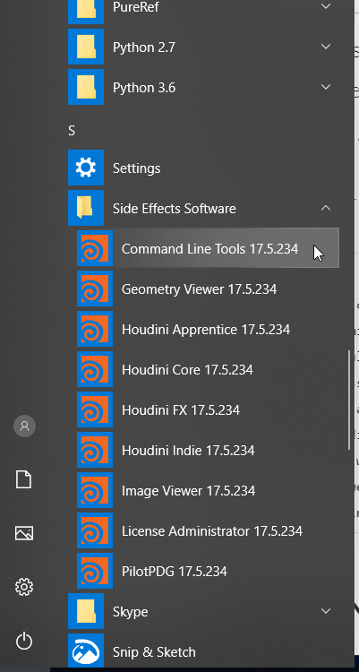
Open Houdini Command Line Tools
Copy SOP_DetailAttrib.c and .h to your project folder
Rename the files.
Rename all references between them inside.
Compile with hcustom
Check if it works in Houdini
The HDK starts with the SOP_Star.c file as an example, but this does not have an input. We want to find the example that is the closest to what we have as possible.
We can grab the SOP_DetailAttrib.c instead. It takes an input and gives an output.

So copy that and SOP_DetailAttrib.h from C:\Program Files\Side Effects Software\Houdini 1x.x.xxx\toolkit\samples\SOP\
and rename them appropriately.
You also want to open the Houdini command line tools, found in your Houdini start folder and navigate to your project folder. This will be how we compile the plugin, instead of in VSCode, as it is both fast and easy.
You can now switch to the houdini commandline again and write hcustom -g SOP_DetailAttrib.c which will compile your code and place it in Houdini.
The starting point should be with as little extra work needed as possible. This might mean that your initial tool will run suboptimal and it might feel amateurish, but the aim should be minimal things that can go wrong.
You might be asking why we are not just using the inlinecpp function, where we pop the C++ into python into Houdini! .. Well… That would in many ways be the obvious choice, so I did that! But several of the debug messages I got were impossible to decipher for me. Imagine, it is Spectra, with Eigen, in HDK, in Python, in Houdini. Things can go wrong.. So it would not have been a bad choice, necessarily, but it turned out to introduce extra levels of uncertainty.
Writing the Plugin
Initial naming and setup
First thing will be to rename the SOP_DetailAttrib .C and SOP_DetailAttrib .h files. I called them SOP_LaplacianEigenExample.C and SOP_LaplacianEigenExample.h.
After this is done, we need to make sure that the C-file can find the header file.
#include "SOP_DetailAttrib.h"
#include "SOP_LaplacianEigenExample.h"
Speaking of includes.. We might as well go ahead and add the includes for Eigen and Spectra. Now, since we have copied it in to where the HDK includes are, this should even work fine with intellisense.
#include <UT/UT_DSOVersion.h>
Notice that I also added #include <iostream> we are going to need to do prints later…
#include <UT/UT_DSOVersion.h>

#include <Eigen/Sparse>
#include <Spectra/MatOp/SparseSymShiftSolve.h>
#include <Spectra/SymEigsShiftSolver.h>
#include <iostream>
Let us also just go ahead and add the namespaces, to make it easier to fill in the code without the namespaces each time. We also don’t need the HDK_Sample namespace.
using namespace HDK_Sample;
And remove in head filer
namespace HDK_Sample {
} // End HDK_Sample namespace
using namespace Eigen;
using namespace Spectra;
using namespace std;
Please note!
This is poor practice, both removing the existing namespace and then adding the other ones.
You might get naming conflicts!
I am doing it here for making it easier and faster to write the code because I already went through and checked that it will work.
Then we need to rename elements in the code, to be sure our classes and functions compile to something uniquely named that does not interfere with what is already in Houdini.
Search for SOP_DetailAttrib and replace it with SOP_LaplacianEigenSolver (or what you choose in both the C-file and header file.
To make it easy to find, we also need to change the name shown to the user.
newSopOperator(OP_OperatorTable *table)
{
    table->addOperator(new OP_Operator(
        "hdk_detailattrib",
        "DetailAttrib",
        SOP_LaplacianEigenExample::myConstructor,
        SOP_LaplacianEigenExample::myTemplateList,
        1,
        1));
}
newSopOperator(OP_OperatorTable *table)
{
    table->addOperator(new OP_Operator(
        "my_laplacianeigensolver",
        "LaplacianEigensolverExample",
        SOP_LaplacianEigenExample::myConstructor,
        SOP_LaplacianEigenExample::myTemplateList,
        1,
        1));
}
.. Now you compile..
.. Because we should make sure that even at this point, things actually work.
Finding the correct includes was a question of finding the correct functions and just go from there.
The example used was gathered from the Spectra and Eigen sites
We only do the naming part because it was the first step to understanding how to set up parameters.
You will be surprised how easily you can make mistakes that you have to backtrack to.
Creating and Filling the Matrix
Let us first find where the actual geometry operations are happening. Try going to line 99.
Here is a function called cookMySop.
Then at line 124, we see an attribute declared. A bit of research shows that this in how we retrieve and modify an attribute.
UT_String aname;
ATTRIBNAME(aname, t);

// Try with a float
GA_RWHandleF attrib(gdp->findFloatTuple(GA_ATTRIB_DETAIL, aname));

// Not present, so create the detail attribute:
if (!attrib.isValid())
    attrib = GA_RWHandleF(gdp->addFloatTuple(GA_ATTRIB_DETAIL, aname, 1));

if (attrib.isValid())
{
    // Store the value in the detail attribute
    // NOTE: The detail is *always* at GA_Offset(0)
    attrib.set(GA_Offset(0), VALUE(t));
    attrib.bumpDataId();
}
We can also find that there are alternative types for the different data types and whether we need arrays. It takes an HDK-specific kind of string called UT_String which is declared separately and called with an odd function called ATTRIBNAME(). We will get back to that.
For now, let us just declare these string types with a normal string as input.
Looking up findFloatTuple() reveals several other methods for getting our attributes.
UT_String aname;
ATTRIBNAME(aname, t);

// Try with a float
GA_RWHandleF attrib(gdp->findFloatTuple(GA_ATTRIB_DETAIL, aname));
UT_String aname;
ATTRIBNAME(aname, t);
UT_String neighboursname = UT_String("neighbours");
UT_String weightsumname = UT_String("weightsum");
UT_String weightsname = UT_String("weights");

GA_RWHandleF attrib(gdp->findFloatTuple(GA_ATTRIB_DETAIL, aname));
GA_RWHandleIA nAttr(gdp->findIntArray(GA_ATTRIB_POINT, neighboursname));
GA_ROHandleF wsAttr(gdp->findFloatTuple(GA_ATTRIB_POINT, weightsumname));
GA_ROHandleFA wAttr(gdp->findFloatArray(GA_ATTRIB_POINT, weightsname));
.. and compile… All good?
… No
Turns out that something is not working, but if we try to change the return type for the second variable, it’s all fine. So change it from GA_ROHandleIA to GA_RWHandleIA .
This might be a good time to also test our result, so after our attribute declarations, add in this code for printing out the first values found
if(nAttr.isValid() && wsAttr.isValid() && wAttr.isValid()) {
    UT_Int32Array nArray;
    UT_FloatArray wArray;
    nAttr.get(0,nArray);
    wAttr.get(0, wArray);
    fpreal32 wsVal = wsAttr.get(0);
    cout << nArray << " " << wArray << " " << wsVal << endl;
}
After compiling, use F5 to start up Houdini through the debugger.
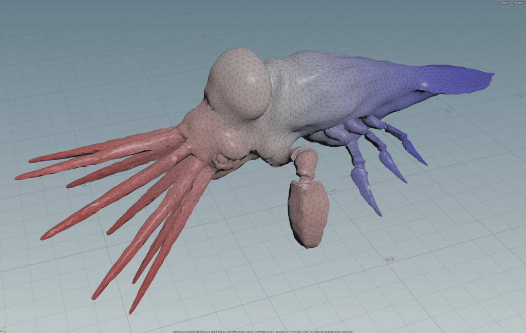
Open our previously set up scene and replace the squab with something lighter, like a box, with a coarser setting on the remesh node.
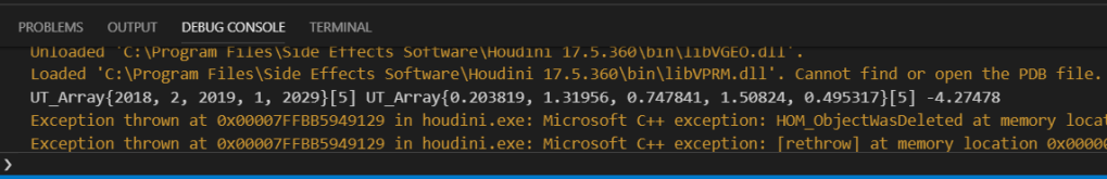
Find your node in the nodes list and plug it in where it belongs.
Now in VSCode you will see, in the Debug Console, the message with the given attributes.
Next up we add the matrix, just before the attribute isValid() check. Finding the syntax in an example on the website for Eigen and the way to get number of points from the HDK reference.
int numPoints = (int)gdp->getNumPoints();
SparseMatrix<double> mat = SparseMatrix<double, RowMajor>(numPoints, numPoints);
We then have to fill the matrix somehow, which would be straight- forward if it was not because Eigen sets requirements for order you fill in the matrix.
A mesh can also have “dead points” when coming into the node, so we can not just iterate from 0 to numpoints, even if we always work with all points. This is why I am using a counter to increment along the point range.
I also utilise a test to check when we have crossed the diagonal, to make sure we do insert in the exactly correct order in the inner loop.
This all adds up to replacing the previous code within the isValid()-test with this:
if(nAttr.isValid() && wsAttr.isValid() && wAttr.isValid()) {
    UT_Int32Array nArray;
    UT_FloatArray wArray;

    GA_Range ptRange = gdp->getPointRange();
    int counter = 0;

    for (GA_Iterator it(ptRange); !it.atEnd(); ++it)
    {
        GA_Offset offset = *it;
        nAttr.get(offset, nArray);
        wAttr.get(offset, wArray);
        fpreal32 wsVal = wsAttr.get(offset);

        bool addingLower = false;
        for (int i = 0; i < nArray.size(); i++)
        {
            if(nArray[i] > counter && !addingLower) {
                mat.insert(counter, counter) = (double)wsVal;
                addingLower = true;
            }
            mat.insert(counter, nArray[i]) = (double)(wArray[i]);
        }
        if (!addingLower) mat.insert(counter, counter) = (double)wsVal;
        counter++;
    }
    cout << mat << endl;
}
Compile and test But be absolutely sure you test with very light geometry! This is an NxN matrix, with all entries being printed. So 1000 points geo will give a million entries!
(You can always kill the process from the VSCode debugger with Shift+F5)
Afterwards, comment out the cout
//cout << mat << endl;
There is a confusing number of functions and variables for such a test.
Luckily, since we have an example, we can ignore anything not obviously necessary to change for now.
The error with the GA_ROHandleIA type not being correct return type is undocumented and an example of where trying to stick closer to the example can resolve your problem.
The auxiliary counter, which just increments for each new occurence in the range, is something that needed a lot of testing. It did not seem like a reliable approach and should not be expected to work.
Especially not when just going 0-numpoints turned out not to work.
Also note that we are creating a large data structure and then tossing it out again each time we cook. This is ineffective, but it is the fastest to figure out.
I have just skipped my own mistakes in the examples above.
For example,
Before using “fpreal32 wsVal = wsAttr.get(0);”,
I also tried just “wsAttr(0, wsVal)”.
Even though this would make little practical sense, it was just what seemed logical.
I chose not to fill the matrix with triplets because it felt unfamiliar and easy to misunderstand.
However, this now meant that care had to be taken in what order the matrix was filled.
I am also used to filling matrices Row-by-row, which also lead to some confusion.
I learned this the hard way, with both crashes and filling the array taking a long time.
I resolved the issue by using timing functions to find out what was taking so long
and finding it was just setting up the matrix,
more than it was the solving.
Luckily, I could just append a “RowMajor” argument, making the code conform to my way of thinking.
Besides that, it was just about writing to the off-diagonal
in the correct order.
So outer loop was going row-by-row,
inner loop column-by-column.
Attributes and Parameters
We need the attributes out in a fashion we can use and we need a parameter to control the number of eigenvectors.
Let us start with the parameters. We could give custom names for the attributes to use, but we will skip that and only do the names we write to. First we change the interface. This means creating some lists of names, defaults and templates.
static PRM_Name	sop_names[] = {
    PRM_Name("attribname",     	"Attribute"),
    PRM_Name("value",      	"Value"),
};

static PRM_Default	sop_valueDefault(0.1);
static PRM_Range	sop_valueRange(PRM_RANGE_RESTRICTED,0,PRM_RANGE_UI,1);

PRM_Template
SOP_LaplacianEigenExample::myTemplateList[]=
{
    PRM_Template(PRM_STRING,1, &sop_names[0], 0),
    PRM_Template(PRM_FLT_J,1, &sop_names[1], &sop_valueDefault, 0,
				   &sop_valueRange),
    PRM_Template()
};
static PRM_Name sop_names[] = {
    PRM_Name("vecattribname", "Eigenvalue Name"),
    PRM_Name("valattribname", "Eigenvector Name"),
    PRM_Name("returncount", "Return Count"),
};

static PRM_Default prm_defaults[] = {
    PRM_Default(0, "eigenVectors"),
    PRM_Default(0, "eigenValues"),
    PRM_Default(4, "")
} ;

static PRM_Range sop_valueRange(PRM_RANGE_RESTRICTED, 2, PRM_RANGE_UI, 100);

PRM_Template SOP_LaplacianEigenExample::myTemplateList[] =
{
        PRM_Template(PRM_STRING, 1, &sop_names[0], &prm_defaults[0]),
        PRM_Template(PRM_STRING, 1, &sop_names[1], &prm_defaults[1]),
        PRM_Template(PRM_INT, 1, &sop_names[2], &prm_defaults[2], 0,
                        &sop_valueRange),
        PRM_Template()
};
And to avoid any errors, we will also need to remove of the actual use of the aname
    // Not present, so create the detail attribute:
    if (!attrib.isValid())
        attrib = GA_RWHandleF(gdp->addFloatTuple(GA_ATTRIB_DETAIL, aname, 1));

    if (attrib.isValid())
    {
        // Store the value in the detail attribute
        // NOTE: The detail is *always* at GA_Offset(0)
        attrib.set(GA_Offset(0), VALUE(t));
        attrib.bumpDataId();
    }
Then under cookMySop() again, find and replace the aname attribute with the strings and integers needed for names of eigenvectors, eigenvalues and number of eigenpairs to generate. Notice that we reference the UI elements by index.
UT_String aname;
ATTRIBNAME(aname, t);

UT_String neighboursname = UT_String("neighbours");
UT_String weightsumname = UT_String("weightsum");
UT_String weightsname = UT_String("weights");

GA_RWHandleF attrib(gdp->findFloatTuple(GA_ATTRIB_DETAIL, aname));
UT_String eVectName;
evalString(eVectName, 0, 0, t);
UT_String eValName;
evalString(eValName, 1, 0, t);
exint eigencount;
eigencount = evalInt(2, 0, t);


UT_String neighboursname ...
After this, we should try to get an output without using the print statement, so we do not end up with a million digits slowly printing to screen. We will just use the “Eigenvectors” attribute for now. Insert this after the matrix-filling loop.
auto matOutAttr = gdp->addFloatArray(GA_ATTRIB_POINT, eVectName, numPoints);
GA_RWHandleFA matOutAttrHandle = GA_RWHandleFA(matOutAttr);
counter = 0;
UT_FloatArray pArray = UT_FloatArray();
pArray.setSize(exint(numPoints));

for (GA_Iterator it(ptRange); !it.atEnd(); ++it)
{
    GA_Offset offset = *it;
    for (int i = 0; i < numPoints; i++)
    {
        pArray[i] = mat.coeff(counter, i);
    }
    matOutAttrHandle.set(offset, pArray);
    counter++;
}
Compile and test!
The Actual solving
At this point, we are ready to pass our matrix through the solver provided by Spectra.
The details on this are readily available on the website.
However, first we need to sanitise our input slightly. We need to make sure we do not try to compute more or less than possible.
if(nAttr.isValid() && wsAttr.isValid() && wAttr.isValid())
int numEigenVs = Index((numPoints - 1 < (int)eigencount ? numPoints - 1 : (int)eigencount));

if(nAttr.isValid() && wsAttr.isValid() && wAttr.isValid() && numPoints >= 2) {
Then after the matrix-filling loop, we want to create the multiplication operator for the matrix (you have this option in case you do your own implementation) and the solver. Then initialise and execute the solving. Add:
Spectra::SparseSymShiftSolve<double> op(mat);
Spectra::SymEigsShiftSolver<double, Spectra::LARGEST_MAGN, Spectra::SparseSymShiftSolve<double>> eigs(&op, numEigenVs, numEigenVs + 1, 0.0);
eigs.init();
eigs.compute();
The choice of solver is based on the documentation.
Now the last thing is writing the whole thing back out.
auto matOutAttr = gdp->addFloatArray(GA_ATTRIB_POINT, eVectName, numPoints);
GA_RWHandleFA matOutAttrHandle = GA_RWHandleFA(matOutAttr);
counter = 0;
UT_FloatArray pArray = UT_FloatArray();
pArray.setSize(exint(numPoints));

for (GA_Iterator it(ptRange); !it.atEnd(); ++it)
{
    GA_Offset offset = *it;
    for (int i = 0; i < numPoints; i++)
    {
        pArray[i] = mat.coeff(counter, i);
    }
    matOutAttrHandle.set(offset, pArray);
    counter++;
}
if (eigs.info() == Spectra::SUCCESSFUL)
{
    VectorXd evalues = eigs.eigenvalues();
    MatrixXd evectors = eigs.eigenvectors();

    int eVectOutSize = (int)evectors.outerSize();
    int eValInSize = (int)evalues.innerSize();

    auto eVectAttr = gdp->addFloatArray(GA_ATTRIB_POINT, eVectName, eVectOutSize);
    GA_RWHandleFA eVectAttrHandle = GA_RWHandleFA(eVectAttr);

    auto eValAttr = gdp->addFloatArray(GA_ATTRIB_DETAIL, eValName, eValInSize);
    GA_RWHandleFA eValAttrHandle = GA_RWHandleFA(eValAttr);
    UT_FloatArray eValArr = UT_FloatArray();

    if (eVectAttrHandle.isValid())
    {
        UT_FloatArray evArr = UT_FloatArray(exint(eVectOutSize));
        evArr.setSize(exint(eVectOutSize));
        counter = 0;
        for (GA_Iterator it(ptRange); !it.atEnd(); ++it)
        {
            GA_Offset offset = *it;
            for (int j = 0; j < eVectOutSize; j++)
            {
                evArr[j] = evectors(counter, j);
            }
            eVectAttrHandle.set(GA_Offset(*it), evArr);
            counter++;
        }
        eVectAttrHandle.bumpDataId();
    }

    if(eValAttrHandle.isValid())
    {
        eValArr.setSize(eValInSize);
        for(int i = 0; i < eValInSize; i++)
        {
            eValArr[i] = evalues[i];
        }
        eValAttrHandle.set(0, eValArr);
        eValAttrHandle.bumpDataId();
    }
}
Compile and test. There. You now got your eigenvectors!
Finding the correct solver for the project took a bit of reading of the documentation.
About how to get the eigenvectors closest to 0
and how to take advantage of the specific matrix type used.
Knowing things like the symmetry of the matrix was helpful.
But it still also took some testing and trying.
Things to optimize:
- Clean up unneeded code in the plugin.
- Getting the vertex area working and switching to a non-symmetric solver
- We should hold on to the matrix in between cooks
- We should look at what is the better solver
- We should implement interrupts and error handling
- Memory management.
What is Next?
So with this new toy, what to do? Don’t worry, there are plenty of papers out there. Plus, the Houdini Gubbins blogs has a multitude of suggestions for topics leaning up against this one.
- Laplacian Mesh Deformation
- Spectral Analysis and Mesh Compression (not that useful)
- Play with poisson or other solvers. Make a Normal > Heightmap converter
- Implement you own solver! a laplacian (non-eigen) solver is fairly straight-forward!
Then you can implement some Navier-Stoke!
You can also use this to get going with a plugin for Houdini, if you need other file formats or libraries.
Thanks To
I had some input early on, before I really understood the concepts, which I really appreciated, so thanks to
Houdini Gubbins blog owner, going by Petz on the Houdini Discord, actually took the time to try and explain a few things.
Likewise, Jake Rice gave a nice long explanation to me on the concept overall.

This is really great stuff man. It’s really hard to find good HDK implementations and breakdowns like this, so it’s awesome to see it all come together. Thanks so much for the shout out as well! Honestly though, this is really inspiring stuff, you should be super proud of what you’ve achieved! 🙂
LikeLike
No worries Jake, appreciate the help 🙂
LikeLike